
FM Synthesis Explained: Linear FM, Through-Zero FM and Exponential FM
What is the difference between linear FM, through-zero FM and exponential FM, and how do they affect the sound spectrum of a synthesizer?
FM Synthesis Explained: Linear FM, Through-Zero FM and Exponential FM
Frequency modulation is one of the most versatile ways to create complex sounds with a synthesizer. It can produce anything from subtle changes in tone to metallic bells, clangorous percussion, evolving drones and spectra that bear little resemblance to the original oscillator waveform.
Yet the term FM synthesis covers several different ways of controlling an oscillator's frequency. Linear FM, through-zero linear FM and exponential FM may use similar-looking patches, but their behaviour can be quite different.
In this article, we'll examine the differences from the perspective of frequency and spectrum. We'll also look at how these techniques can be explored using Cherry Audio Voltage Modular's Zeroscillator.
1. What happens in frequency modulation?
Let's begin with two oscillators.
The first oscillator produces the sound we want to hear. It is commonly called the carrier. The second oscillator, called the modulator, controls the carrier's instantaneous frequency.
Instead of remaining at a constant frequency, the carrier speeds up and slows down according to the modulator's signal.
For example, imagine a carrier tuned to 220 Hz and a modulator producing a sine wave at 55 Hz. If the modulation is relatively shallow, the carrier's frequency will move up and down around its nominal value. If the modulation becomes stronger, the resulting waveform becomes more complex, and the sound spectrum can expand considerably.
The crucial point is that the spectrum of an FM sound is not determined by the carrier frequency alone. It also depends on the modulator frequency, the modulation depth, and the way the modulator affects the carrier.
When the modulator operates at audio rate, the resulting spectrum can contain many additional frequency components called sidebands. These can lie above and below the carrier frequency and, at sufficient modulation depths, become more prominent than the carrier itself.
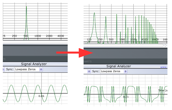
This is why FM can transform a simple sine wave into a sound with a rich, complicated spectrum.
2. Carrier frequency, modulator frequency and sidebands
Let's use a simple sinusoidal modulator.
If the carrier frequency is (f_c) and the modulator frequency is (f_m), the main sideband frequencies occur at intervals related to the modulator frequency:
[
f_c \pm f_m,\quad f_c \pm 2f_m,\quad f_c \pm 3f_m,\ldots
]
These are the potential sideband locations. Their amplitudes are not all equal, and some may be extremely weak or absent depending on the modulation index.
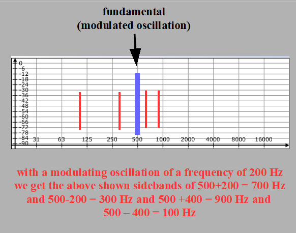
For example, with a carrier at 220 Hz and a modulator at 55 Hz, the first sideband pair lies at 165 Hz and 275 Hz. The next pair lies at 110 Hz and 330 Hz, followed by 55 Hz and 385 Hz.
This is a simplified illustration of the possible sideband positions. The actual spectrum depends on the modulation depth, and some components may have zero or negligible amplitude.
The relationship between carrier and modulator frequencies is important.
If the frequencies have a simple integer ratio, the resulting components can align with a harmonic series associated with a common fundamental. Depending on the ratio and the strength of the sidebands, this can produce a pitched, harmonic or bell-like sound.
If the relationship is more complicated, the sidebands may not align neatly with one harmonic series. The result can sound metallic, clangorous or inharmonic.
Try changing only the modulator frequency while keeping the carrier frequency and modulation depth fixed. You will hear that the sound can change substantially even though the carrier itself has not been retuned.
3. Modulation depth and the FM index
The amount of frequency variation matters just as much as the frequencies involved.
For sinusoidal FM, a useful theoretical quantity is the modulation index, commonly represented by the Greek letter beta ((\beta)). For ideal sinusoidal frequency modulation, it is the peak frequency deviation divided by the modulator frequency:
[
\beta = \frac{\Delta f}{f_m}
]
Here, (\Delta f) is the peak frequency deviation and (f_m) is the modulator frequency.
In practical terms, the modulation index helps describe how much sideband energy is generated relative to the carrier. As the index increases, more sidebands can become significant, often producing a more complex spectrum.
This does not mean that increasing the index simply makes every frequency component louder. Individual sidebands change in amplitude in a more complicated way. Some may grow while others shrink, and particular components can disappear at certain index values.
On the Zeroscillator, the FM INDEX input and its associated controls provide ways to influence the effective depth of the modulation coming through the MODULATOR route. This makes it possible to shape the spectrum dynamically rather than keeping the modulation depth fixed.
An envelope controlling FM INDEX, for example, can produce a bright, complex attack that becomes smoother as the modulation depth decreases.
This is one of the most useful techniques to experiment with when designing percussive FM sounds.
4. Linear FM: frequency changes in a linear relationship
With linear frequency modulation, the modulating signal affects the carrier's instantaneous frequency in a linear relationship. Equal changes in the modulation signal produce equal changes in frequency, provided the modulation scaling remains constant.
In an idealised model, the instantaneous frequency can be expressed as:
[
f_i(t) = f_c + k,m(t)
]
Here, (f_c) is the carrier's nominal frequency, (m(t)) is the modulating signal and (k) determines the modulation sensitivity.
When the modulator is a sine wave, the carrier frequency moves above and below its nominal value in a sinusoidal pattern.
Linear FM is particularly useful when you want the modulation to behave predictably in terms of frequency deviation. It also forms the basis of many classic digital FM synthesis techniques.
However, there is an important practical distinction between a linear frequency relationship and the ability to pass through zero frequency. A linear modulation signal does not automatically imply that the oscillator can run backwards. That depends on how the oscillator handles frequencies at and below zero.
This leads us to through-zero FM.
5. Through-zero linear FM: what happens at zero?
In through-zero linear FM, the instantaneous frequency is allowed to pass through zero and become negative.
When the instantaneous frequency is positive, the oscillator's phase progresses in its usual direction. At zero frequency, the phase progression momentarily stops. When the frequency becomes negative, the phase progresses in the opposite direction.
This reversal is the defining feature of through-zero FM.
Imagine a carrier whose nominal frequency is 100 Hz. A sufficiently strong linear modulating signal might drive its instantaneous frequency down to zero and then into negative values during part of the modulation cycle.
An oscillator that supports through-zero operation can represent this behaviour directly. An oscillator that does not support it must handle the zero crossing differently, for example by preventing the frequency from becoming negative or by applying another internal response.
Those different behaviours can produce different waveforms and spectra.
Why can through-zero FM sound different?
When the oscillator reverses its phase progression, the resulting waveform differs from one whose frequency is simply constrained to remain positive. This can affect the spectrum and the way timbre changes with modulation depth.
Through-zero FM can be especially useful when exploring deep linear modulation, where the instantaneous frequency may repeatedly cross zero.
It is not a guarantee of a particular sound. The result still depends on the carrier frequency, modulator frequency, modulation depth and waveform shapes. Some settings produce subtle differences; others produce dramatically different timbres.
Try it on the Zeroscillator
Load a basic two-oscillator FM patch in Voltage Modular and keep the tuning, modulator and modulation depth unchanged.
Switch between TYPICAL and THROUGH ZERO modes. Then increase the modulation depth gradually.
Listen to the spectral changes, especially as the modulation becomes deep enough to produce reverse phase progression in through-zero mode.
To understand the difference, avoid changing several other controls at the same time. A consistent comparison makes it easier to identify what the through-zero switch is doing.
6. Exponential FM: a different relationship
The Zeroscillator also provides exponential FM inputs.
With exponential frequency control, the incoming voltage affects frequency through an exponential relationship rather than a linear one. This is the principle behind conventional volt-per-octave pitch control: a change of one volt corresponds to an octave when the input is calibrated for 1 V/oct.
This distinction becomes particularly important when the input receives an audio-rate modulating signal rather than a slowly changing pitch CV.
With linear FM, a given modulation amplitude produces a given frequency deviation in hertz. With exponential FM, the effect is multiplicative: equal changes in control voltage correspond to frequency ratios rather than equal changes in hertz.
Consequently, exponential FM can behave differently as the carrier's nominal pitch changes. The same modulating voltage can produce a different absolute frequency deviation at different carrier frequencies.
This can make exponential FM particularly useful for exploring pitch-dependent timbral changes, but it also means its behaviour should not be assumed to match linear FM.
Using the Zeroscillator's exponential inputs
The Zeroscillator has a 1V/OCT input for conventional pitch control, as well as two additional inputs labelled EXP FM 1 and EXP FM 2.
The 1V/OCT input is useful for playing melodic sequences. Its attenuator changes the pitch scaling, so the usual one-volt-per-octave relationship applies only at the appropriate setting.
EXP FM 1 and EXP FM 2 have bidirectional attenuators. Near their centre positions, the modulation is reduced to zero; turning the controls to opposite sides of centre reverses the modulation polarity.
Try patching the same waveform into both EXP FM inputs and setting their attenuators to opposing positions. With suitably matched signals and settings, the modulation effects can cancel. Then use different waveforms or different amplitudes to explore how the two inputs combine.
This is a practical way to investigate the interaction between exponential modulation signals.
7. Linear FM versus exponential FM
The following table summarises the main distinction.
| Feature | Linear FM | Exponential FM |
|---|---|---|
| Relationship between control and frequency | Linear frequency deviation | Exponential frequency relationship |
| Equal changes in control signal | Equal changes in frequency, for a fixed linear scaling | Equal changes in control voltage correspond to frequency ratios |
| Behaviour when carrier pitch changes | Frequency deviation can remain fixed for a fixed modulation amplitude | Absolute frequency deviation generally changes with carrier pitch |
| Through-zero behaviour | Possible if the oscillator supports negative instantaneous frequency | Not implied by exponential FM |
| Typical uses | Controlled frequency deviation and FM-spectrum experiments | Pitch-related modulation and pitch-dependent timbral changes |
Neither approach is universally better. They are different tools, and their usefulness depends on the sound you want to create.
Also, the labels on a synthesizer's controls describe how the modulation is implemented, not a guaranteed sound category. Linear FM can sound harmonic or inharmonic, smooth or aggressive. Exponential FM can also create a broad range of timbres.
8. Why the modulator waveform matters
So far, we've mainly considered sinusoidal modulation because it makes the frequency relationships easier to describe. In practice, the modulator can have many different shapes.
A sine wave provides a smooth, continuously changing modulation signal. A square wave changes abruptly between levels. A sawtooth or ramp waveform sweeps in one direction before returning to its starting value.
These different shapes have different spectral contents. When used as audio-rate modulators, they can generate different families of spectral components and produce different changes in timbre.
The Zeroscillator allows you to use different waveforms and morph continuously between triangle, sine and square. This gives you a way to change the modulation signal's character while the patch is running.
Try the following experiment:
- Set up a simple linear FM patch.
- Start with a sine-wave modulator.
- Keep the carrier pitch and modulation depth fixed.
- Change the modulator to a triangle wave.
- Try a square wave and then a ramp or sawtooth.
- Compare the results at both shallow and deep modulation depths.
Then try morphing between waveforms while the FM patch plays. You will hear the spectrum evolve as the modulation source changes.
The resulting sound is not simply a blend of the spectra of the original waveforms. The modulator changes the carrier's instantaneous frequency, so the relationship between the signals is what generates the resulting spectral structure.
9. Practical experiment: create a moving FM spectrum
Here is a useful patching exercise that combines several of the ideas discussed in this article.
You will need:
- Two oscillators, with one acting as the carrier and one as the modulator.
- A way to control modulation depth, such as an attenuator or envelope.
- An audio output.
- Optional: a spectrum analyser or oscilloscope.
Patch and explore:
- Send the modulator's audio output to the carrier's linear FM input.
- Route the carrier to your audio output.
- Start with a relatively low modulation depth.
- Adjust the modulator frequency and listen for changes in the spectrum.
- Increase the modulation depth gradually.
- If the carrier supports through-zero FM, compare through-zero and conventional linear operation.
- Replace the sine modulator with other waveforms.
- Use an envelope to change modulation depth over the course of a note.
Finally, use the spectrum analyser if you have one. Watch how the distribution of spectral energy changes as you adjust the modulator frequency and modulation index.
You can also use a slow LFO or envelope to control the modulation depth over a longer period. This creates evolving timbres without requiring the carrier's pitch to change.
10. Where to go next with the Zeroscillator
The Zeroscillator is particularly useful because it combines linear FM, through-zero linear FM, exponential FM, PWM, TIME REVERSAL and wave morphing in one module.
These functions allow you to investigate not only how frequency modulation works, but how it interacts with waveform shape, phase relationships and control signals.
For practical examples, continue with Patch Lab: Four Voltage Modular Zeroscillator Experiments. That article explores basic FM with envelope control, morphing as a modulation source, two-oscillator patches and stereo morphing.
For a closer look at the module's controls and signal routing, read The Voltage Modular Zeroscillator Explained: FM, Through-Zero FM and Wave Morphing.
The larger lesson is that FM is not a single sound or technique. It is a family of ways to control frequency, and the results depend on the mathematical relationship between the carrier, the modulator and the modulation depth. Once you understand those relationships, you can use FM more deliberately—or use them as a starting point for sound-design experiments whose results are not entirely predictable.